fit

iris.sg.background.fit(data, velocity, axis_wavelength, where=True)

Compute the parameters of model_total() which best fit data using the gradient descent method.

Parameters:

• data (AbstractScalar) – The observation to be fitted.

• velocity (AbstractScalar) – The Doppler velocity for each point in the observation

• axis_wavelength (str) – The logical axis corresponding to increasing wavelength (velocity).

• where (bool | AbstractScalar) – The points in the observation to consider when fitting.

Return type:

CartesianNdVectorArray

Examples

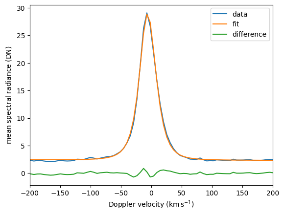
Fit a spectrograph image and display the average actual line profile compared to the average fitted line profile.

import numpy as np
import matplotlib.pyplot as plt
import astropy.units as u
import astropy.visualization
import named_arrays as na
import iris

# Load a spectrograph observation
obs = iris.sg.SpectrographObservation.from_time_range(
    time_start=astropy.time.Time("2021-09-23T06:00"),
    time_stop=astropy.time.Time("2021-09-23T07:00"),
)

# Save the time and raster axes
axis = (obs.axis_time, obs.axis_detector_x)

# Compute the average along the time and raster axes
avg = iris.sg.background.average(
    obs=obs,
    axis=axis,
)

# Ignore line profiles that are mostly NaN
where_crop = np.isfinite(avg.outputs).mean(avg.axis_wavelength) > 0.7
data = avg.outputs[where_crop]

# Convert wavelength to velocity units
velocity = avg.inputs.velocity.cell_centers()
velocity = velocity[where_crop]

# Fit the data within +/- 150 km/s of line center
where = np.abs(velocity) < 150 * u.km / u.s
parameters = iris.sg.background.fit(
    data=data,
    velocity=velocity,
    axis_wavelength=obs.axis_wavelength,
    where=where,
)

# Evaluate the model with the best-fit parameters
data_fit = iris.sg.background.model_total(
    velocity=velocity,
    amplitude=parameters.components["amplitude"],
    shift=parameters.components["shift"],
    width=parameters.components["width"],
    kappa=parameters.components["kappa"],
    bias=parameters.components["bias"],
    slope=parameters.components["slope"],
)

# Plot the average data and model
with astropy.visualization.quantity_support():
    fig, ax = plt.subplots()
    na.plt.plot(
        velocity.mean(obs.axis_detector_y),
        data.mean(obs.axis_detector_y),
        label="data",
    )
    na.plt.plot(
        velocity.mean(obs.axis_detector_y),
        data_fit.mean(obs.axis_detector_y),
        label="fit",
    )
    na.plt.plot(
        velocity.mean(obs.axis_detector_y),
        (data - data_fit).mean(obs.axis_detector_y),
        label="difference"
    )
    ax.set_xlim(-200, 200)
    ax.set_xlabel(f"Doppler velocity ({ax.get_xlabel()})")
    ax.set_ylabel(f"mean spectral radiance ({ax.get_ylabel()})")
    ax.legend();