estimate

iris.sg.background.estimate(obs, axis_time, axis_wavelength, axis_detector_x, axis_detector_y)

Estimate the background from a given spectrograph observation.

This function applies average(), subtract_spectral_line(), and smooth() in succession to estimate the background.

Parameters:

• obs (SpectrographObservation) – The observation to estimate the background from.

• axis_time (str) – The logical axis corresponding to changing raster number.

• axis_wavelength (str) – The logical axis corresponding to changing wavelength.

• axis_detector_x (str) – The logical axis corresponding the changing position perpendicular to the slit.

• axis_detector_y (str) – The logical axis corresponding to changing position along the slit.

Return type:

SpectrographObservation

Examples

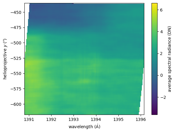
Estimate the background from a spectrograph observation

import numpy as np
import matplotlib.pyplot as plt
import astropy.units as u
import astropy.visualization
import named_arrays as na
import iris

# Load a spectrograph observation
obs = iris.sg.SpectrographObservation.from_time_range(
    time_start=astropy.time.Time("2021-09-23T06:00"),
    time_stop=astropy.time.Time("2021-09-23T07:00"),
)

# Subtract the spectral line from the average
bg = iris.sg.background.estimate(
    obs=obs,
    axis_time=obs.axis_time,
    axis_wavelength=obs.axis_wavelength,
    axis_detector_x=obs.axis_detector_x,
    axis_detector_y=obs.axis_detector_y,
)

# Plot the result
with astropy.visualization.quantity_support():
    fig, ax = plt.subplots()
    img = na.plt.pcolormesh(
        bg.inputs.wavelength,
        bg.inputs.position.y,
        C=bg.outputs.value,
    )
    ax.set_xlabel(f"wavelength ({ax.get_xlabel()})")
    ax.set_ylabel(f"helioprojective $y$ ({ax.get_ylabel()})")
    fig.colorbar(
        mappable=img.ndarray.item(),
        ax=ax,
        label=f"average spectral radiance ({obs.outputs.unit})",
    )

Subtract the background from the observation and compare to the original.

# Remove background from spectrograph observation
obs_nobg = obs.copy_shallow()
obs_nobg.outputs = obs.outputs - bg.outputs

# Select the first raster to plot
index = {obs.axis_time: 0}

# Plot the original compared to the background-subtracted
# observation.
with astropy.visualization.quantity_support():
    fig, ax = plt.subplots(
        ncols=2,
        sharex=True,
        sharey=True,
        constrained_layout=True,
    )
    mappable = plt.cm.ScalarMappable(
        norm=plt.Normalize(vmin=0, vmax=5),
    )
    ax[0].set_title("original")
    na.plt.pcolormesh(
        obs.inputs.position.x[index],
        obs.inputs.position.y[index],
        C=np.nanmean(obs.outputs.value[index], axis=obs.axis_wavelength),
        ax=ax[0],
        norm=mappable.norm,
        cmap=mappable.cmap,
    )
    ax[1].set_title("corrected")
    na.plt.pcolormesh(
        obs_nobg.inputs.position.x[index],
        obs_nobg.inputs.position.y[index],
        C=np.nanmean(obs_nobg.outputs.value[index], axis=obs.axis_wavelength),
        ax=ax[1],
        norm=mappable.norm,
        cmap=mappable.cmap,
    )
    ax[0].set_xlabel(f"helioprojective $x$ ({ax[0].get_xlabel()})")
    ax[0].set_ylabel(f"helioprojective $y$ ({ax[0].get_ylabel()})")
    fig.colorbar(
        mappable=mappable,
        ax=ax,
        label=f"mean spectral radiance ({obs.outputs.unit:latex_inline})",
    )

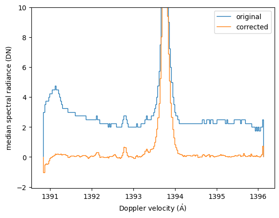
Plot the original and corrected median spectral line profiles

# Define the axes to average over
axis_txy = (
    obs.axis_time,
    obs.axis_detector_x,
    obs.axis_detector_y,
)

# Plot the result
with astropy.visualization.quantity_support():
    fig, ax = plt.subplots()
    na.plt.stairs(
        obs.inputs.wavelength.mean(obs.axis_time),
        np.nanmedian(obs.outputs, axis=axis_txy),
        label="original",
    )
    na.plt.stairs(
        obs_nobg.inputs.wavelength.mean(obs.axis_time),
        np.nanmedian(obs_nobg.outputs, axis=axis_txy),
        label="corrected",
    )
    ax.set_xlabel(f"Doppler velocity ({ax.get_xlabel()})")
    ax.set_ylabel(f"median spectral radiance ({ax.get_ylabel()})")
    ax.set_ylim(top=10)
    ax.legend()